Note. This tutorial's interactive widgets and its citation previews require JavaScript to be enabled in your browser.
If you were to ask seven radiologists to outline the same structure on the same medical image, it is almost a certainty that you will get seven different masks. To someone unfamiliar with medical imaging, this might seem like carelessness, but it is not. Boundaries in medical images are genuinely ambiguous, and if you add personal annotation preferences or “style”, expertise levels, and other factors, the disagreement starts to make sense. Across organs and modalities, the volume of a manually contoured structure routinely varies by tens of percent between observers (for example, inter-observer volume differences of 20% and more are common in CT organ delineation), and that variation propagates directly into downstream tasks: radiotherapy decisions, measurements, and the “ground truth” on which segmentation models are trained and evaluated. When these annotations feed a supervised model, the choice of how to collapse them into a single training target is a modeling decision, and this tutorial shows how different methods can make that decision differently.
Unfortunately, resources on this topic are scarce, and I am aware of only one other tutorial on this topic. We will talk about five families of consensus methods, from counting votes to a learned expectation-maximisation (EM) procedure, and run all of them on two deliberately dissimilar datasets. The first is the QUBIQ 2021 brain-growth task, in which seven expert segmentations of a developing brain structure on T1-weighted MRI(volumetric and grayscale), and the clinical quantity of interest is a volume that changes slowly over time, so a systematic bias in the consensus may lead to a systematic bias in the growth curve. The second is IMA++, in which five annotators outline skin-lesion boundaries in 2D RGB dermoscopic images, and the boundary decisions affect downstream melanoma-risk features.
All visualizations here are produced by a single notebook (linked at the end) that runs on CPU in a couple of minutes. The key code is inline so that you can follow along as you read.
The “problem”
It is important to visualize how this disagreement presents, especially when you are new to this topic. In the widget below, toggle individual raters on and off over the image, hover to magnify both panels together, and watch the vote countmap on the right (the number of raters who called each pixel foreground). Here, I present two more tasks from the QUBIQ dataset: kidney CT (three raters) and prostate MRI (six raters). Hopefully, this helps you appreciate the ubiquity of annotator disagreement. The methods in this post are run only on the brain MRI and the dermoscopy case alone, but as you will see, they are very straightforward to apply to other datasets.
A few quick observations:
- The annotators generally agree on the interior. Almost all of the disagreement lives in a thin band at the boundary.
- The shape of the disagreement is modality-specific: on the brain MRI, the raters argue about a diffuse, low-contrast edge; on the dermoscopy image, they argue about how far a pigmented region reaches into visually similar skin; on the kidney CT, where soft-tissue contrast is comparatively high, they agree closely and differ only along the organ rim; on the prostate MRI, they disagree more sharply about how far a zone with no crisp boundary extends.
Majority voting and mask averaging
The vote count map above already suggests the simplest possible rule.
Consider the per-pixel decision in isolation: if at least half of the $K$ raters marked a pixel as foreground, keep it. That is majority voting (MV): simply thresholding the vote count map at $K/2$. And if instead of thresholding, if you retain the fraction, you get mask averaging (MA), a soft consensus in the interval $[0, 1]$ that doubles as a crude per-pixel confidence. The code for both is straightforward:
import numpy as np

def majority_vote(masks):            # masks: (K, H, W) uint8
    # Ties go to foreground: a pixel needs >= K/2 votes, so with K = 6 a
    # 3-3 split is kept. This inclusive convention biases the consensus
    # very slightly towards larger structures.
    return (masks.sum(0) >= masks.shape[0] / 2).astype(np.uint8)

def mask_average(masks):
    return masks.mean(0, dtype=np.float32)
Majority voting is fast, parameter-free, and a good baseline when annotators are of comparable skill. It has two structural weaknesses, both of which follow from its treating every rater as equally reliable and deciding each pixel independently: it cannot tell a careful/skilled annotator from a careless/less-skilled one, and it can leave an isolated speck in the consensus wherever a bare majority of raters happened to overlap on a stray patch (circled below, left; click to zoom).
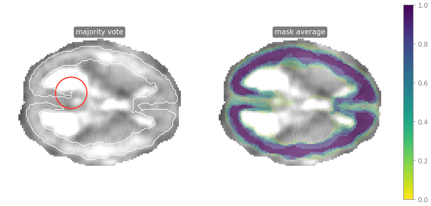
These are the two good starting points because they represent opposite extremes: MV decides too early (thresholding) and MV never decides (soft consensus). All the other methods that follow are more principled and nuanced ways to turn disagreement into a single mask. And the first question we need to ask is whether all raters truly deserve an equal vote.
Takeaway: MV is a good first baseline and very fast to compute, but it is blind to rater skill.
STAPLE
Consider a realistic annotation setup: a senior radiologist, a junior resident both delineate the same tumour. The resident is not wrong so much as systematically generous, consistently including a few millimetres of healthy tissue (a very realistic setting as shown in a study of 12 dermatologists), so we need to account for this to not let their bias leak into the final consensus. We would like to estimate how reliable each rater is and weight them accordingly, and this is what the very popular STAPLE (Simultaneous Truth And Performance Level Estimation) does.
Let $x_t \in \lbrace 0, 1 \rbrace$ denote the unknown true label at voxel $t$, and let $y_{it}$ denote the label rater $i$ assigned to that voxel. Each rater is modelled as a noisy channel described by two numbers: a sensitivity $\theta_{i1} = p(y_{it} = 1 \mid x_t = 1)$ (i.e., how much of the true foreground the rater captures) and a specificity $\theta_{i0} = p(y_{it} = 0 \mid x_t = 0)$ (i.e., how well the rater excludes true background). Assuming the raters annotate independently given the truth, the likelihood of their labels at a voxel factorises over raters:
$$ p(y_t \mid x_t = a; \theta) = \prod_{i=1}^{m} p(y_{it} \mid x_t = a; \theta_{ia}), \qquad a \in \lbrace 0, 1 \rbrace $$
The consensus is then found by expectation-maximisation (EM), which alternates between estimating the truth and evaluating the raters. In the E-step, the current performance estimates and a prior foreground probability $p_{\text{prior}}$ are combined by Bayes’ rule into the posterior probability that a voxel is truly foreground:
$$ w_t(1) = \frac{p_{\text{prior}} \prod_i p(y_{it} \mid x_t = 1)}{p_{\text{prior}} \prod_i p(y_{it} \mid x_t = 1) + (1 - p_{\text{prior}}) \prod_i p(y_{it} \mid x_t = 0)} $$
In the M-step, those soft assignments re-estimate each rater, sensitivity from the voxels the consensus now believes are foreground and specificity from the rest:
$$ \theta_{i1} = \frac{\sum_t y_{it} w_t(1)}{\sum_t w_t(1)}, \qquad \theta_{i0} = \frac{\sum_t (1 - y_{it}) w_t(0)}{\sum_t w_t(0)} $$
with $w_t(0) = 1 - w_t(1)$. The two steps iterate to convergence, and a reliable rater ends up moving the consensus far more than an unreliable one. We use SimpleITK’s STAPLEImageFilter to run STAPLE and extract the per-rater performance estimates.
import SimpleITK as sitk

def run_staple(masks):               # masks: (K, H, W) uint8
    imgs = [sitk.Cast(sitk.GetImageFromArray(m), sitk.sitkUInt8)
            for m in masks]
    f = sitk.STAPLEImageFilter(); f.SetForegroundValue(1)
    soft = sitk.GetArrayFromImage(f.Execute(imgs))
    # In SimpleITK 2.4.1 these take NO index and return all K values at once.
    return (soft.astype("float32"),
            np.array(f.GetSensitivity()),
            np.array(f.GetSpecificity()))
On the QUBIQ case, the estimated sensitivities spread the seven raters across an appreciable range (0.695 to 0.820), and plotting sensitivity against specificity shows who tends to over-segment (high sensitivity, low specificity) and who tends to under-segment, as shown below.
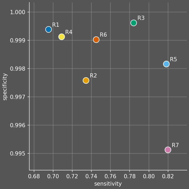
One key thing to note is that because specificity is a true-negative rate estimated over the background, the amount of background you give STAPLE changes the estimate. Our QUBIQ frame is roughly 90% black padding (empty background), so if you run STAPLE on the full frame, every rater’s specificity is close to 1. If you crop tightly around the structure (toggle to “Tight crop” below), things change.
Running STAPLE on the full frame yields a consensus of 2,939 pixels, but the tight crop’s consensus is only of 2,569 pixels, which is a difference of about 13%. So in a way, the background extent is a hyperparameter for STAPLE.
Takeaway: STAPLE is a good choice when raters differ in skill, but it is important to factor in the background extent.
SIMPLE
While STAPLE re-weights raters, it never completely discards one. This distinction is important when working with large-scale or crowdsourced annotations, where some raters may be unreliable, and STAPLE would still include their masks as evidence. SIMPLE (Selective and Iterative Method for Performance Level Estimation), on the other hand, takes a more decisive approach by filtering out raters outright: it estimates a consensus, scores each rater against it, discards the raters whose agreement is too low, and repeats this process until the consensus stabilises.
Concretely, at iteration $j$, SIMPLE forms an estimate $E^{(j)}$, scores each rater by their overlap with that estimate, and retains a rater only while their score stays within a fixed multiple of the spread of the panel:
$$ \phi_i = \operatorname{DSC}(S^i, E^{(j)}), \qquad \text{keep rater } i \iff \phi_i \ge \bar{\phi} - \lambda \sigma_{\phi} $$
where $S^i$ is rater $i$’s mask, $\operatorname{DSC}$ is the Dice coefficient, $\bar{\phi}$ and $\sigma_{\phi}$ are the mean and standard deviation of the scores across the surviving raters, and $\lambda$ is a rejection threshold. “Bad” annotators are voted off rather than down-weighted. We can use the SIMPLE implementation from FeTS-AI’s LabelFusion.
from LabelFusion.wrapper import fuse_images

def run_simple(masks):               # masks: (K, H, W) uint8
    imgs = [sitk.Cast(sitk.GetImageFromArray(m), sitk.sitkUInt8)
            for m in masks]
    fused = fuse_images(imgs, "simple", class_list=[0, 1])
    return sitk.GetArrayFromImage(fused)
In any large annotation project, it is common to end up with empty masks. STAPLE handles this gracefully though. In the QUBIQ case, the 2,939-pixel consensus from seven raters would not change if an eighth rater submitted a blank mask. EM would push the empty rater’s sensitivity to zero and specificity to one.
On the other hand, correlated errors are a problem for STAPLE. STAPLE assumes independent errors given the true label, so shared biases, e.g., multiple raters systematically submitting generous segmentation masks (i.e., over-segmenting) because of a shared tool or protocol will affect STAPLE’s estimates. We can see this in the hypothetical scenario below:
| panel | $K$ | MV | STAPLE | SIMPLE |
|---|---|---|---|---|
| seven real raters | 7 | 2,246 | 2,939 | 2,246 |
| + 1 generous | 8 | 2,569 | 2,939 | 2,246 |
| + 3 generous (colluding) | 10 | 2,939 | 8,241 | 2,569 |
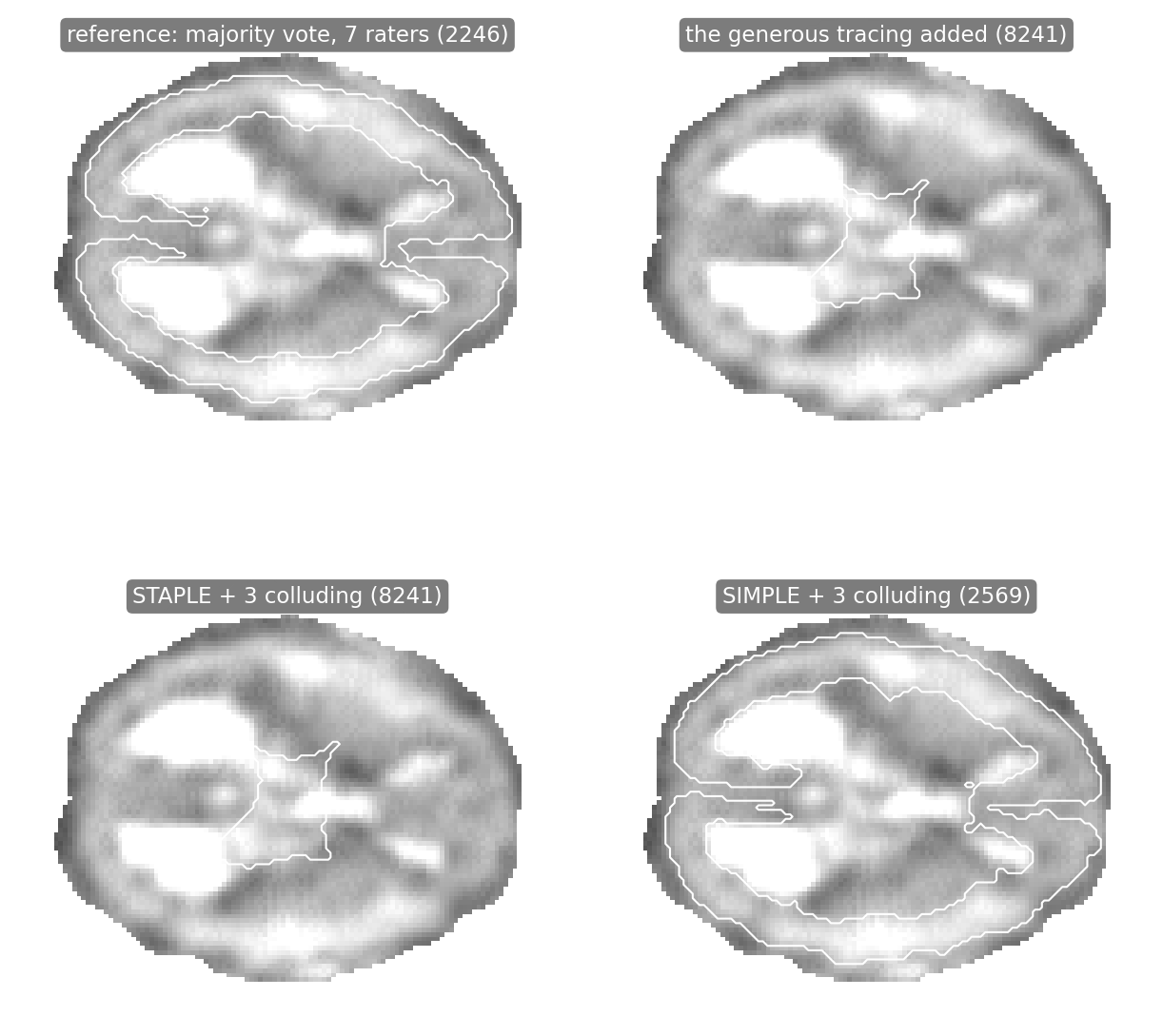
The 8,241-pixel consensus from STAPLE is striking, and unsurprisingly, the exact size of the “generous” tracing itself. STAPLE completely adopts the generous tracing, thus (erroneously) concluding that three annotators who agree perfectly with one another are the reliable ones and that the seven who disagree with them are not. On the other hand, SIMPLE scores each rater against its current estimate, spots the three generous raters as outliers, and returns an almost unaffected consensus of 2,569 pixels.
This is also why SIMPLE just returns the majority vote on perfectly clean data (row 1), because if it does not need to reject any raters, the final step is simply a vote among the remaining raters. When the data is “contaminated”, a single generous rater moves majority voting by 14% (row 2), but SIMPLE is unaffected.
Takeaway: Both STAPLE and SIMPLE are robust to a single bad annotator, but when a group of raters is systematically bad, SIMPLE is more robust due to its rejection step.
MACCHIatO
Unlike the previous methods that have all been probabilistic, MACCHIatO (Morphologically-Aware Consensus Computation via Heuristics-based IterATive Optimization) treats consensus as a geometric problem. This is especially useful when the final output needs to be a well-formed, cohesive mask instead of just an arbitrary collection of individual pixels. Let $S^1, \ldots, S^K$ denote the $K$ rater masks, each a binary labelling of the $N$ pixels, and let $M \in \lbrace 0, 1 \rbrace^N$ be any candidate consensus. Instead of counting votes, MACCHIatO defines the consensus $T$ as the Fréchet mean under a chosen distance, i.e., the single mask $T$ that minimises the average (squared) distance to all rater masks. Using the Dice-based distance,
$$ T = \arg\min_{M \in \lbrace 0,1 \rbrace^N} \frac{1}{K}\sum_{k=1}^{K} \bigl(1 - \operatorname{DSC}(M, S^k)\bigr)^2 $$
where $\operatorname{DSC}$ is the Dice similarity coefficient. To visualize how this works, imagine stacking all the raters’ masks on top of each other. The algorithm organizes the pixels (voxels) into crowns, i.e., sets of voxels that share the same global morphological distance from the intersection of all the raters’ masks. These are further divided into subcrowns based on which specific group of raters segmented them. MACCHIatO iteratively “peels” these subcrowns awat from the outside going inwards, thus removing the weakest agreement first.
As MACCHIatO peels away these low-agreement subcrowns, the objective function drops until it reaches a minimum, and then starts increasing again if you start to remove the high-agreement core. Play with the interactive widget below to see how the consensus changes as you peel away the subcrowns, watching how stepping through the peeling process changes the objective function, and the minimum is achieved at step 3. You will notice that the descent is not always perfectly monotonic, and it might even go back up slightly before finding the minimum, and this is why the algorithm searches for the absolutely minimum rather than stopping when the objective stops improving.
We can use the Hard_MACCHIatO function from the paper’s official code repository to compute the MACCHIatO consensus:
from macchiato.hard_consensus import Hard_MACCHIatO
from macchiato.utils import soft_dice          # our Dice-based distance

masks_list = [masks[k].astype(float) for k in range(len(masks))]
consensus = Hard_MACCHIatO(masks_list, dist=soft_dice, verbose=False)
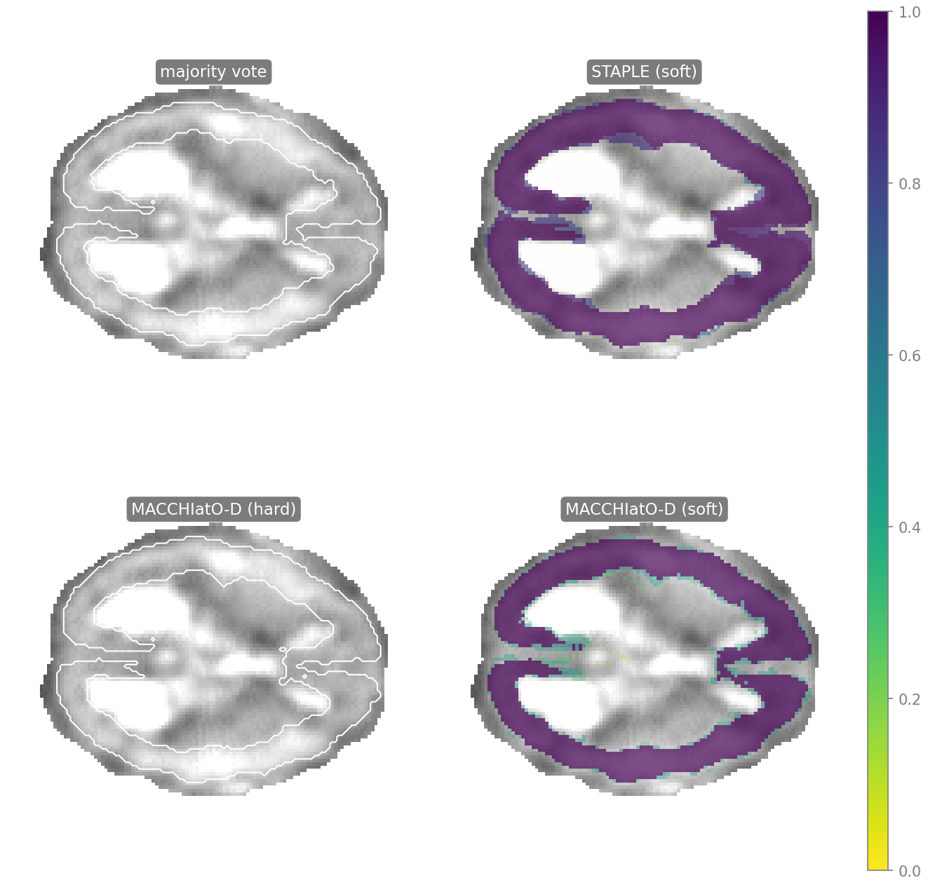
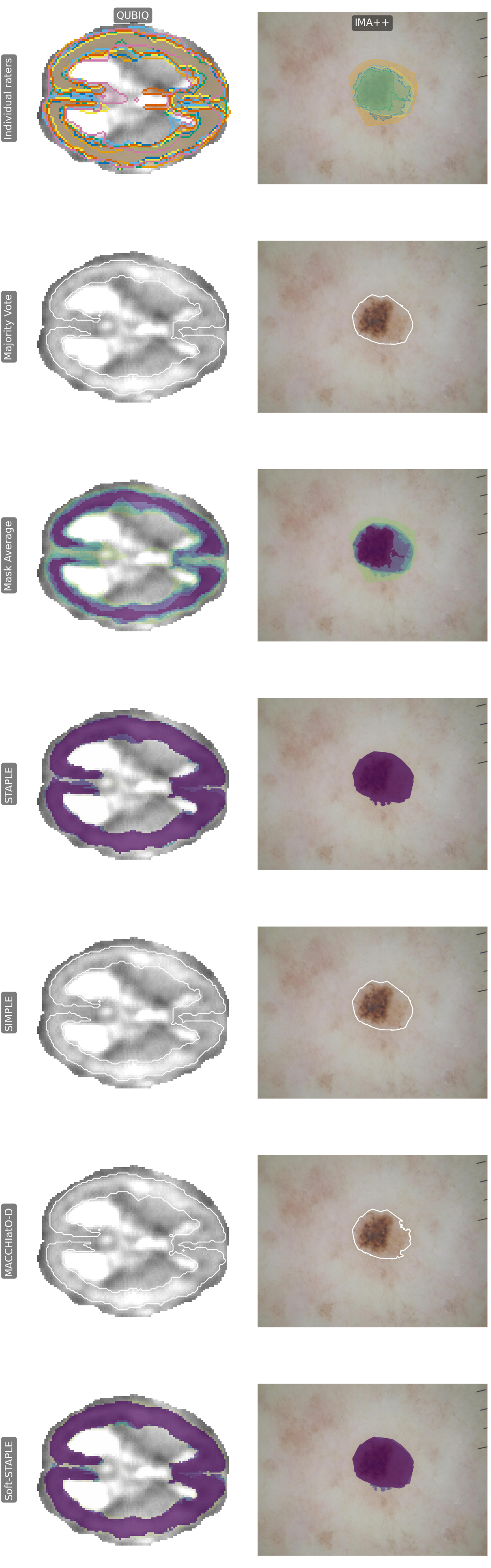
MACCHIatO has a surprising property: because it optimizes overlap globally rather than voting pixel-by-pixel, MACCHIatO’s hard consensus is not bounded below by MV. When the raters disagree strongly, it can return a smaller mask than MV. The reason is that since Dice is a ratio, adding a peripheral pixel that only a minority of raters marked increases the mask size (denominator) for every rater. So when the union gets large and the pairwise overlaps are still small, the penalty for growing the mask dominates, and so the optimiser drops the pixel. You can see this in the combined results in the combined results below. On the concordant QUBIQ case, MACCHIatO lands just above MV, but on the high-disagreement IMA++ case, its consensus (42,265 px) falls below majority vote (44,795 px). The only guarantee is that it never exceeds the union.
Takeaway: MACCHIatO produces a consensus that is optimal in an explicit, reportable sense (the Fréchet mean), rather than as the by-product of a voting rule. The tradeoff, however, is heavier computation and a consensus size that seem counter-intuitive to the “more agreement means larger” intuition.
Soft-STAPLE
Every method we have looked at so far assumes raters provide strictly binary masks. However, a rater’s confidence is rarely uniform across an outline, especially at the edges. For example, when segmenting malignant lesions in dermoscopy images, structures like pseudopods exhibit high uncertainty, and their presence itself is clinically significant and informative of the diagnosis,, so that uncertainty is useful. Soft-STAPLE handles this by accepting soft annotations, allowing boundary uncertainty to be processed as input.
Now let each rater provide a soft opinion $q_{it}(b) = p(y_{it} = b)$ for $b \in \lbrace 0, 1 \rbrace$, and write $q_{it} \equiv q_{it}(1)$ for the soft foreground weight. The objective is the expected log-likelihood under those soft opinions, $L_{\text{soft}}(\theta) = \sum_t \mathbb{E}_{q_t}[\log p(y_t; \theta)]$, and the resulting E-step weight is an expectation over the raters’ opinions,
$$ w_t(a) = \sum_{B \in \lbrace 0,1 \rbrace^m} q_t(B), p(x_t = a \mid y_t = B; \theta) $$
where $B$ ranges over all joint labellings of the $m$ raters. Note that this sum scales exponentially with the number of raters, so it is much more practical to use the paper’s “simplified” variant, which just blends a rater’s sensitivity and error rate using their soft score:
$$ p(y_{it} \mid x_t = 1; \theta) = q_{it} \theta_{i1} + (1 - q_{it})(1 - \theta_{i1}) ,$$
and similarly for the background. You can verify that if you feed binary inputs to this expression, it reduces to standard STAPLE.
For the purposes of this tutorial, since we only have binary masks, we choose to synthesize soft inputs. The original paper did this in a modality-specific manner by dilating the binary mask and keeping only the added voxels that hit a certain MRI intensity threshold (FLAIR-hyperintense), but that was because they only evaluated it on one dataset. We want our approach to be modality-agnostic so that it works both on brain MRIs and dermoscopic images, and so we simply use pure morphological dilation, giving the newly added “rim” a fractional weight.
from skimage.morphology import binary_dilation, disk

def generate_soft_labels(mask, radius=3, weight=0.3):
    core = mask > 0
    rim  = binary_dilation(core, disk(radius)) ^ core
    soft = core.astype("float32")
    soft[rim] = weight            # boundary voxels: uncertain, not absent
    return soft
This approach introduces two crucial parameters that significantly affect the final consensus mask shape: the rim radius $r$ (i.e., the spatial extent of the boundary uncertainty) and the weight $w$ (i.e., the assigned probability within that uncertain region). If you use a narrow, faint rim ($r=3$, $w=0.3$), the consensus is practically identical to standard STAPLE (2,915 versus 2,939 pixels), and the uncertain band is barely visible. But if you widen this band and increase the uncertainty weight ($r=8$, $w=0.5$), the “graded” band now occupies 4% of the image, and the consensus’ size grows considerably to 3,409 pixels.
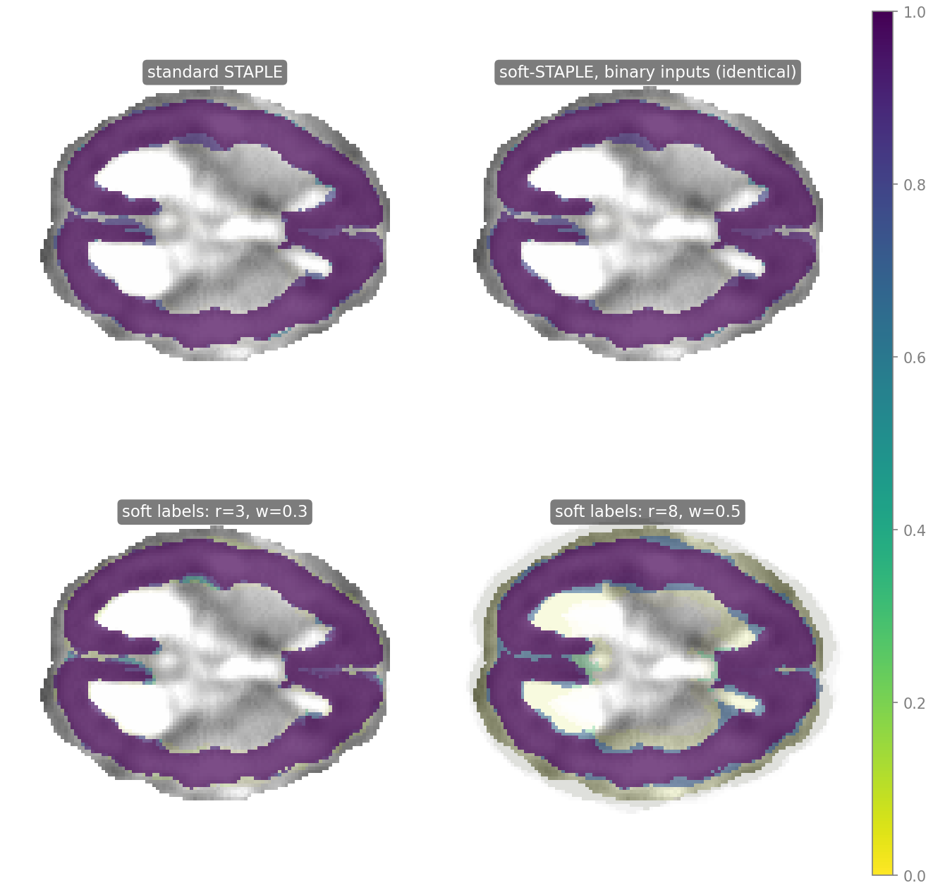
Takeaway: If the raters can explicitly map their boundary uncertainty (the typical scenario with deep learning models’ segmentation predictions), Soft-STAPLE is a mathematically elegant way to fuse them. But if the uncertainty is synthesized after the fact (like here), the design choices are important and should also be reported transparently.
Choosing among them
These five algorithm families answer different questions, and the right choice usually boils down to what you know about your annotators and what your downstream task needs. These methods’ summaries and their trade-offs are listed in the table below. After that, an interactive figure lets you compare every method on both the datasets. You will notice that for the dermoscopy image, the annotators disagree about the lesion’s extent by arguably a clinically meaningful margin.
| Method | What it models | Handles an unreliable rater? | Soft output? | Key assumption / caveat |
|---|---|---|---|---|
| Majority Vote / Mask Average | pixel-wise vote count | no (equal weight) | MA only | none; fast baseline |
| STAPLE | per-rater sensitivity + specificity | down-weights, never removes | yes | background extent is a parameter |
| SIMPLE | consensus + iterative rater rejection | yes, removes outliers | no (hard label) | a rejection threshold $\lambda$ |
| MACCHIatO-D | Fréchet mean under Dice | implicitly, via the mean | yes | heavier optimisation; size can fall below MV |
| Soft-STAPLE | STAPLE on soft annotations | down-weights | yes | needs soft labels (here, we synthesise them by dilation) |
Should you collapse the raters at all?
Every method we have discussed here reduces many annotations to one mask, and in doing so, discards the disagreement, which has unsurprisingly been shown to be meaningful,. Consensus aggregation is perfect when you genuinely need a single “gold standard” ground truth mask, which is often, but not always. So, instead of collapsing that variability, you could:
- Sample the variance: use a Probabilistic U-Net to generate plausible segmentations that match the observed variability.
- Disentangle bias: utilize a label-noise framework to disentangle each annotator’s bias from the underlying “ground truth” while training.
- Predict preferences: train your model to explicitly predict individual raters’ specific decisions.
- Discover styles: learn the underlying segmentation “styles” that form the basis of the inter-rater variability in the first place.
Your turn
So far, you have been watching these methods run on fixed data. Perhaps the best way to understand how a single annotator influences the final mask is … to become one. The interactive widget below shows a dermoscopy image (ISIC_0000432) featuring a faint lesion with an ambiguous boundary. Trace a single closed loop exactly where you think the boundary lies, and click “Calculate consensus”. It will show you how two raters outlined the exact same lesion, and it will compute MV, MA, STAPLE with you as Rater 3. You can toggle R1/R2’s masks, but I would suggest you draw your own boundary before you see theirs.
Notice how the two raters drew smooth contours that cross each other, meaning each rater includes a region that the other excludes. So they disagree on where the lesion ends, and aggregation methods we discussed here aim to resolve exactly these kinds of boundary ambiguities. And as you play around with this, I want you to pay attention to the STAPLE estimates. If you draw a careful contour that aligns with the experts, your sensitivity and specificity scores will be high. If you draw something hasty, empty, or wildly over-inclusive, STAPLE will quietly down-weight your reliability, reducing your influence on the final consensus. So the mask you obtain is a function of the raters and the method together, and here one of the raters is you.
Code and notebooks
All visualizations here are produced by a single Jupyter notebook that runs entirely on CPU in a couple of minutes. The notebook and a small, tested, accompanying Python library are available at github.com/kakumarabhishek/segmentation-consensus-tutorial, with a requirements.txt. We used the Dice-based distance for MACCHIatO throughout the code because it is the metric most readers are familiar with. However, switching to the Jaccard variant is just a one-line change.
Note: The QUBIQ and IMA++ datasets are not redistributed, so you will need to point the notebook to your own local copies of these datasets.
References
- Joskowicz et al. Inter-observer variability of manual contour delineation of structures in CT. European Radiology 29, 2019. [DOI]
- Li et al. QUBIQ: Uncertainty Quantification for Biomedical Image Segmentation Challenge. arXiv:2405.18435, 2024. [DOI]
- Abhishek et al. IMA++: ISIC Archive Multi-Annotator Dermoscopic Skin Lesion Segmentation Dataset. IEEE Data Descriptions 3, 2026. [DOI]
- Fortina et al. Where's the naevus? Inter‐operator variability in the localization of melanocytic lesion border. Skin Research and Technology 18 (3), 2012. [DOI]
- Warfield et al. Simultaneous Truth and Performance Level Estimation (STAPLE): An Algorithm for the Validation of Image Segmentation. IEEE Transactions on Medical Imaging 23(7), 2004. [DOI]
- Langerak et al. Label Fusion in Atlas-Based Segmentation Using a Selective and Iterative Method for Performance Level Estimation (SIMPLE). IEEE Transactions on Medical Imaging 29(12), 2010. [DOI]
- Hamzaoui et al. Morphologically-Aware Consensus Computation via Heuristics-based IterATive Optimization (MACCHIatO). Machine Learning for Biomedical Imaging (MELBA) 2:013, 2023. [DOI]
- Kittler et al. Chaos and Clues. Dermoscopedia. [URL]
- Menzies et al. The Morphologic Criteria of the Pseudopod in Surface Microscopy. JAMA Dermatology 131 (4), 1995. [DOI]
- Williams et al. Assessment of Diagnostic Accuracy of Dermoscopic Structures and Patterns Used in Melanoma Detection: A Systematic Review and Meta-analysis. JAMA Dermatology 157 (9), 2021. [DOI]
- Kats et al. A Soft STAPLE Algorithm Combined with Anatomical Knowledge. MICCAI, 2019. [DOI]
- Cheplygina et al. Crowd Disagreement About Medical Images Is Informative. MICCAI LABELS, 2018. [DOI]
- Abhishek et al. What Can We Learn from Inter-Annotator Variability in Skin Lesion Segmentation?. MICCAI ISIC, 2025. [DOI]
- Kohl et al. A Probabilistic U-Net for Segmentation of Ambiguous Images. NeurIPS, 2018. [URL]
- Zhang et al. Disentangling Human Error from the Ground Truth in Segmentation of Medical Images. NeurIPS, 2020. [URL]
- Ji et al. Learning Calibrated Medical Image Segmentation via Multi-rater Agreement Modeling. CVPR, 2021. [DOI]
- Abhishek et al. Segmentation Style Discovery: Application to Skin Lesion Images. MICCAI ISIC, 2024. [DOI]